
DDAS Machine Insight Suite – Understanding Your Data
About this guide
The library manuals describe every function block, input and output. This guide answers a different question: what do the numbers tell you? It explains the information you get from the Machine Insight Suite, shows with worked examples how the values relate to each other, and points out what to check when a value looks unexpected.
It is written for machine builders who integrate the suite, and for the people who read the results on a dashboard: production managers, process engineers and operators.
The OEE terms and formulas follow the widely used definitions published on oee.com (Vorne Industries). Where the suite deviates from them or adds something, this guide says so.
| You want to know | Chapter |
|---|---|
| Which information the suite provides and where it comes from | 2 |
| What a "schedule" is and why everything is counted per schedule | 3 |
| How the time of a shift is divided into productive time and losses | 4 |
| How OEE, availability, performance, quality and TEEP are calculated | 5 |
| How stops are classified and what short stops are | 6 |
| What targets, throughput and losses in product count mean | 7 |
| How to read the top 10 stop reasons | 8 |
| How the batch end time is forecast | 9 |
| How several shifts or batches are combined | 10 |
| Why a value looks different from what you expected | 11 |
Document history
| Version | Date | Author | Description |
|---|---|---|---|
| 1.0 | 07.10.2026 | DDAS | Initial version |
| 1.1 | 08.10.2026 | DDAS | Time model: note that the speed loss is updated with each counted part. |
The information at a glance
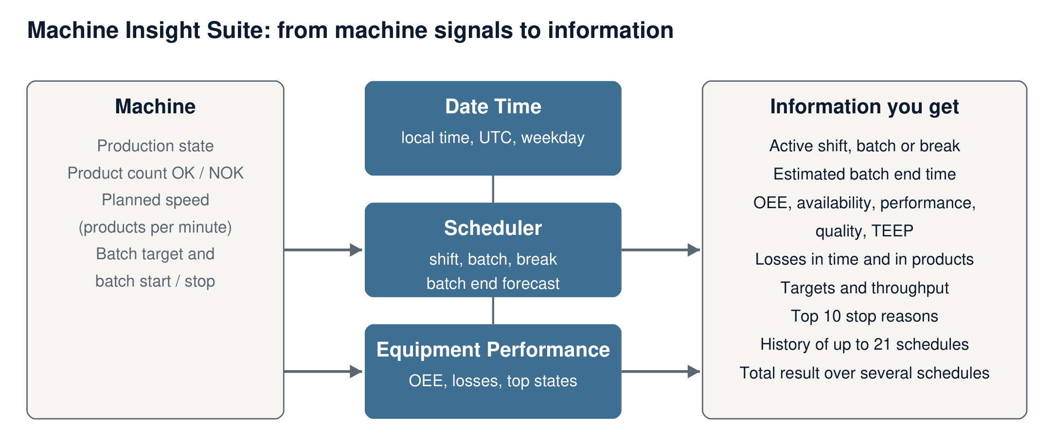
The suite needs only a few signals from the machine. From these it derives all information:
| Signal from the machine | Used for |
|---|---|
| Production state (producing, starved, blocked, no material, operator stop, failure, not ready, no demand) | Losses, availability, top states |
| Product count OK and NOK | Quantity, quality, performance, throughput |
| Planned speed in products per minute | Ideal cycle time, targets, performance |
| Batch target, batch start and stop | Batch end forecast |
| Shift and break calendar (parameters) | Active schedule, planned production time |
| Information | Provided by | Structure |
|---|---|---|
| Local time, UTC time, weekday, calendar week | Date Time Library | scDateTimeInfo |
| Active shift, batch or break with start and end | Scheduler Library, GetSchedule | scScheduleInfo |
| Remaining build time and estimated batch end | Scheduler Library, GetBuildTime and GetBatchScheduledEndTime | — |
| OEE, availability, performance, quality, TEEP, quantities, targets, throughput | Equipment Performance Library | scPerformanceDetails |
| Production times of the schedule | Equipment Performance Library | scProductionDetails |
| Duration and number of every kind of stop | Equipment Performance Library | scProductionLossDetails |
| Top 10 stop reasons by duration and by occurrence | Equipment Performance Library | scTopState |
| The last 21 schedules | EP_History | arrays of the structures above |
| One total result over several schedules | EP_Result | scEP_Result |
All values are calculated on the controller, in every PLC cycle. They are available without a database or a cloud connection and can be shown on a visualization or passed on to a higher-level system.
Everything is counted per schedule
A schedule is the period for which the suite collects and evaluates data. It can be
a shift from the weekly shift calendar,
a batch, started and stopped by the machine program, or
a product run, when a second instance evaluates each product separately.
When a schedule starts, all counters start at zero. When it ends, the result is frozen, can be stored in the history, and the next schedule starts again at zero. Every value in this guide therefore answers the question "how is this shift (or batch) doing so far?", not "how is the machine doing in general?". Chapter 10 shows how to combine several schedules.
A break does not end a schedule. It pauses it: during a planned break no stop is counted and the time is not part of the planned production time.
Good to know
Parts that the machine produces while no schedule is active are not lost. They are added to the quantity of the next schedule and count for its quality, but they do not improve its performance or throughput.
Two shifts that follow each other without a gap are evaluated separately.
A schedule can be evaluated for up to 49 days.
The time model
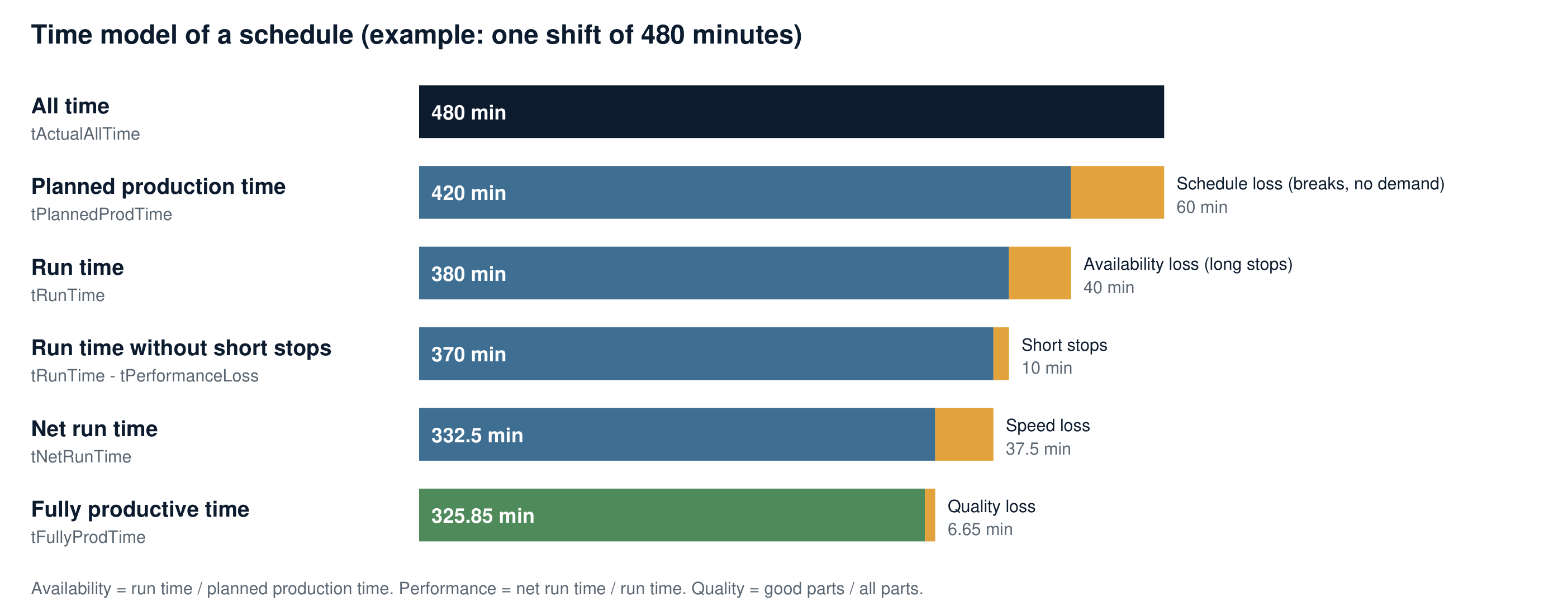
OEE divides the time of a schedule into what was productive and what was lost, step by step. The suite provides every step as a value.
| Step | Meaning | Value |
|---|---|---|
| All time | Time since the schedule started | scPD.tActualAllTime |
| − Schedule loss | Time in which no production was planned: breaks, "no demand" and time without a reported state | scEP.tScheduleLoss |
| = Planned production time | Time in which the machine should have produced | scPD.tPlannedProdTime |
| − Availability loss | Long stops: failure, not ready, and every stop longer than the short stop time | scEP.tAvailabilityLoss |
| = Run time | Time in which the machine was running | scPD.tRunTime |
| − Short stops | Stops shorter than the short stop time | scEP.tPerformanceLoss |
| − Speed loss | Time lost because the machine ran slower than planned | scEP.tSpeedLoss |
| = Net run time | Time the produced parts need at planned speed (ideal cycle time × total count) | scPD.tNetRunTime |
| − Quality loss | Time spent on rejected parts | scEP.tQualityLoss |
| = Fully productive time | Time spent on good parts at planned speed | scPD.tFullyProdTime |
Where the suite gives you more detail than the standard model
The standard model has one performance loss. The suite splits it into short stops (measured as time) and speed loss (calculated: the part of the run time that is neither a short stop nor net run time). You can see at once whether the machine loses output by stopping briefly or by running slowly. The performance loss of the standard model is the sum of both.
The time model adds up: tRunTime = tPerformanceLoss + tSpeedLoss + tNetRunTime. The speed loss is updated with each counted part, so between two parts the sum can differ by up to one cycle time. Its ratios can be checked directly: performance is tNetRunTime / tRunTime, quality is tFullyProdTime / tNetRunTime, and OEE is tFullyProdTime / tPlannedProdTime.
OEE and its three factors
Formulas
| KPI | Formula | Question it answers |
|---|---|---|
| Availability | Run time / Planned production time | How much of the planned time was the machine running? |
| Performance | (Ideal cycle time × Total count) / Run time | How fast did it run while it was running? |
| Quality | Good count / Total count | How many of the parts were good? |
| OEE | Availability × Performance × Quality | How much of the planned time was fully productive? |
| TEEP | OEE × Planned production time / All time | How much of the whole time was fully productive? |
Ideal cycle time is the time for one product at planned speed: 60 s / products per minute. With 60 products per minute it is 1 s. The suite calls it rProductTime.
Worked example
One shift, the same numbers as in the figure of chapter 4:
| Input | Value |
|---|---|
| Shift length | 480 min |
| Breaks | 60 min |
| Long stops | 40 min |
| Short stops | 10 min |
| Planned speed | 60 products per minute, ideal cycle time 1 s |
| Total count | 19,950 products |
| Rejected (NOK) | 399 products |
| Step | Calculation | Result |
|---|---|---|
| Planned production time | 480 − 60 | 420 min |
| Run time | 420 − 40 | 380 min = 22,800 s |
| Good count | 19,950 − 399 | 19,551 |
| Availability | 380 / 420 | 90.4 % |
| Performance | (1 s × 19,950) / 22,800 s | 87.5 % |
| Quality | 19,551 / 19,950 | 98.0 % |
| OEE | 0.9047 × 0.875 × 0.98 | 77.5 % |
| TEEP | 77.58 % × 420 / 480 | 67.8 % |
The suite cuts the percentages after one decimal place; it does not round up. 90.47 % is shown as 90.4 %.
Check: in this example OEE can also be calculated directly as (good count × ideal cycle time) / planned production time = 19,551 s / 25,200 s = 77.5 %. Both ways give the same result, and the three factors show in addition where the 22 % were lost.
This shortcut works only as long as the ideal cycle time stays the same. As soon as the product changes during a schedule and the new product has a different planned speed, there is no single cycle time to multiply the count with. The suite therefore does not use the shortcut. It weights every part with the cycle time that was valid when the part was produced and calculates the performance from this sum (chapter 5.4). The result is correct for one product and for any number of product changes.
Example: a shift runs 200 minutes with product A (60 per minute, cycle time 1 s) and produces 10,800 parts, then 180 minutes with product B (30 per minute, cycle time 2 s) and produces 4,860 parts. The net run time is 10,800 × 1 s + 4,860 × 2 s = 20,520 s = 342 min. With a run time of 380 min the performance is 342 / 380 = 90.0 %. Multiplying the total of 15,660 parts with either of the two cycle times would give 68.7 % or 137.4 %, both wrong.
How to read the result
OEE is a product. Three factors of 90 % give an OEE of only 73 %. A low OEE with three "good" factors is normal.
Look at the trend, not at the absolute value. oee.com names 85 % as world class for discrete manufacturing (90 % availability, 90 % performance, 99 % quality) and around 60 % as typical. These numbers are a reference, not a target for every machine. A realistic target is one you can reach within a few months.
OEE and TEEP answer different questions. OEE judges the time in which production was planned. TEEP also counts breaks and "no demand" against the machine and shows how much capacity is left. In the suite, "all time" is the time since the schedule started. TEEP is therefore the utilization within this shift or batch; time between two schedules is not part of it.
A performance above 100 % means that the planned speed is set lower than the speed the machine actually reaches. Check the value of products per minute.
What the suite does in addition
| Behaviour | Why | Setting |
|---|---|---|
| Performance is shown as 100 % at the start of a schedule | With the first few parts the value would jump between extremes | Start-up time and start-up count in scPar (default 5 min and 10 parts) |
| KPIs are refreshed every few seconds, not in every cycle | A calm display that an operator can read | scPar.tKPIUpdateFilter (default 5 s) |
| The planned speed may change during a schedule | Each part is weighted with the cycle time that was valid when it was produced, so a product change does not distort the performance | Input rProductsPerMin |
| OEE is 0 as long as one factor is 0 | Before the first part, quality and performance are not defined | — |
Stops and losses
Which state causes which loss
The machine program reports one production state at a time. The suite assigns it to a loss:
| Production state | Typical cause | Loss | OEE factor |
|---|---|---|---|
| Producing | Machine is running | none | — |
| NoDemand | No order, waiting for start | Schedule loss | not part of OEE |
| Break (from the schedule) | Planned break | Schedule loss | not part of OEE |
| None | The machine program reports no state (error 32) | Schedule loss | not part of OEE |
| Starved | No parts from upstream | short: performance loss, long: availability loss | Performance / Availability |
| Blocked | Downstream does not take parts | short: performance loss, long: availability loss | Performance / Availability |
| NoMaterial | Material ran out | short: performance loss, long: availability loss | Performance / Availability |
| OperatorStop | Operator stops for a minor issue | short: performance loss, long: availability loss | Performance / Availability |
| EquipmentFailure | Fault, emergency stop | Availability loss | Availability |
| NotReady | Stopped, waiting for restart | Availability loss | Availability |
How your machine states map to these states is defined once in the machine program (function StateConverter in the Application Template). This mapping decides how meaningful the result is. If, for example, every stop is reported as NotReady, the OEE is still correct, but the loss analysis and the top states cannot tell you anything.
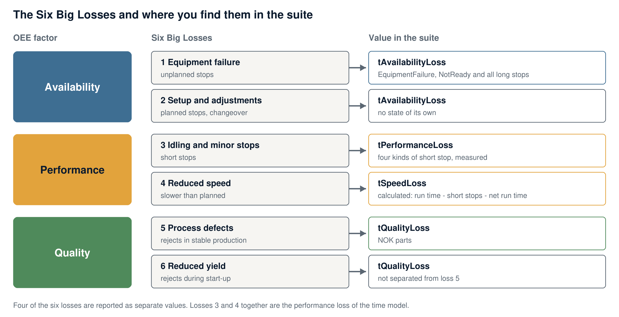
Relation to the "Six Big Losses" (oee.com):
| Six Big Losses | In the suite |
|---|---|
| Equipment failure (unplanned stops) | EquipmentFailure, NotReady and the long stops |
| Setup and adjustments (planned stops) | Reported by your machine program as one of the states; as NoDemand it is a schedule loss, as NotReady or OperatorStop an availability loss |
| Idling and minor stops | The four short stops |
| Reduced speed | Speed loss |
| Process defects, reduced yield | Quality loss (NOK parts); the suite does not separate start-up rejects from production rejects |
The suite reports four of the six losses as separate values. The time model of oee.com combines "idling and minor stops" and "reduced speed" into one performance loss; in the suite this is tPerformanceLoss + tSpeedLoss. The speed loss is calculated, not measured: everything that slows the machine down without being reported as a stop ends up there. Between two parts it rises slightly and falls back when the next part is counted.
Short stops
A machine that stops forty times for five seconds has a different problem than a machine that stands once for three minutes. The suite therefore separates short stops from long stops.
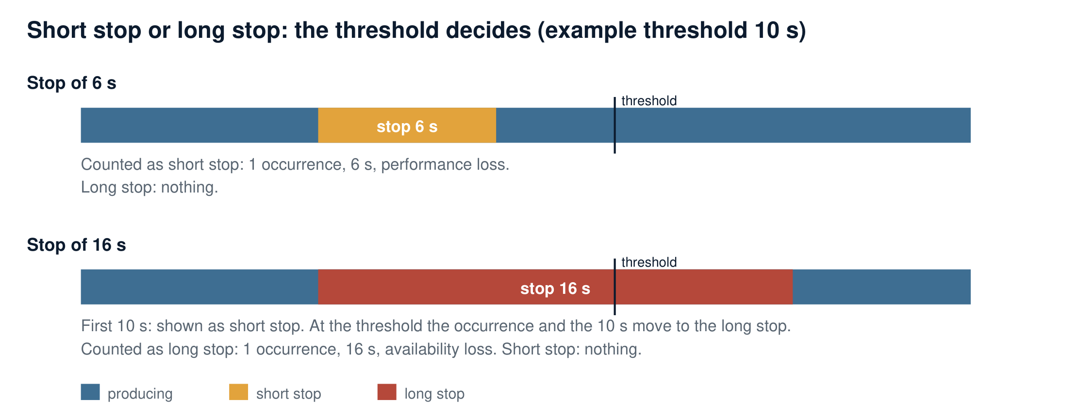
You set the limit: tShortStopTimePerfLoss for Starved, Blocked and NoMaterial (default 10 s) and tShortStopTimeAvailLoss for OperatorStop (default 30 s).
Every stop is counted once, with one occurrence and its whole duration, either as a short stop or as a long stop.
While a stop is running and has not yet reached the limit, you see it as a short stop. At the limit it moves to the long stop, together with the time that has passed. At this moment the performance loss goes down and the availability loss goes up by the same amount. This is intended.
EquipmentFailure and NotReady are always long stops.
Choosing the limit: oee.com describes minor stops as stops of a minute or two that the operator resolves without maintenance. The defaults of the suite are lower, because a PLC can measure much shorter stops than a person can log. Set the limit to the duration below which nobody on your shop floor would write down a reason.
What you get for every kind of stop
For each of the ten kinds of stop (six long, four short), for breaks, NoDemand and the state None, scProductionLossDetails provides the total duration and the number of occurrences. tUnplannedDowntime and uiUnplannedOccurrence are the totals of the ten kinds of stop.
Duration divided by occurrences gives the average length of a stop. A long average points to a repair or supply problem, a short average with many occurrences to a chronic disturbance.
Targets, throughput and losses in products
Time is exact, but "we lost 40 minutes" is abstract. The suite therefore also expresses the result in products.
Targets
| Value | Formula | Meaning |
|---|---|---|
| lrActualPlanTarget | Planned production time / ideal cycle time | Products you would have by now without any loss |
| lrActualNetTarget | Run time / ideal cycle time | Products you would have by now if the machine had run at planned speed whenever it ran |
| lrActualPlanOEETarget | lrActualPlanTarget × OEE target | Products you should have by now at your target OEE |
| lrActualNetOEETarget | lrActualNetTarget × OEE target | The same, based on the run time |
The targets grow with time. They show where the schedule should be right now, not at its end. Compare them with lrQuantity: if the quantity is above the OEE target, the shift is ahead of plan. The OEE target is the input rOEEpercent.
Throughput
| Value | Formula | Meaning |
|---|---|---|
| lrActualPlanTPH | Quantity / planned production time, per hour | Real output per planned hour |
| lrTargetPlanTPH | lrActualPlanTarget / planned production time, per hour | Planned output per hour |
| lrActualNetTPH | Quantity / run time, per hour | Real output per hour of running |
| lrTargetNetTPH | lrActualNetTarget / run time, per hour | Planned output per hour of running |
The plan throughput includes all stops and answers "how much do we really get per hour?". The net throughput leaves out the long stops and answers "how fast is the machine when it runs?".
Losses in products
| Value | Formula |
|---|---|
| lrScheduleLoss | Schedule loss / ideal cycle time |
| lrAvailabilityLoss | Availability loss / ideal cycle time |
| lrPerformanceLoss | Short stops / ideal cycle time |
| lrQualityLoss | Number of NOK parts |
| lrSpeedLoss | Speed loss / ideal cycle time |
The example in products
| Value | Calculation | Result |
|---|---|---|
| Plan target | 420 min × 60 | 25,200 |
| Quantity | 19,950 | |
| Availability loss | 40 min × 60 | 2,400 |
| Performance loss (short stops) | 10 min × 60 | 600 |
| Speed loss | 25,200 − 19,950 − 2,400 − 600 | 2,250 (= 37.5 min) |
| Quality loss | 399 | |
| Plan target at 85 % OEE target | 25,200 × 0.85 | 21,420 |
| Actual plan throughput | 19,950 / 7 h | 2,850 per hour |
| Target plan throughput | 25,200 / 7 h | 3,600 per hour |
| Actual net throughput | 19,950 / 6.33 h | 3,150 per hour |
Reading: the shift is 5,250 products behind the ideal. 2,400 were lost in long stops, 600 in short stops and 2,250 because the machine ran slower than planned. With a target of 85 % the shift should have 21,420 products and is 1,470 behind.
Top 10 stop reasons
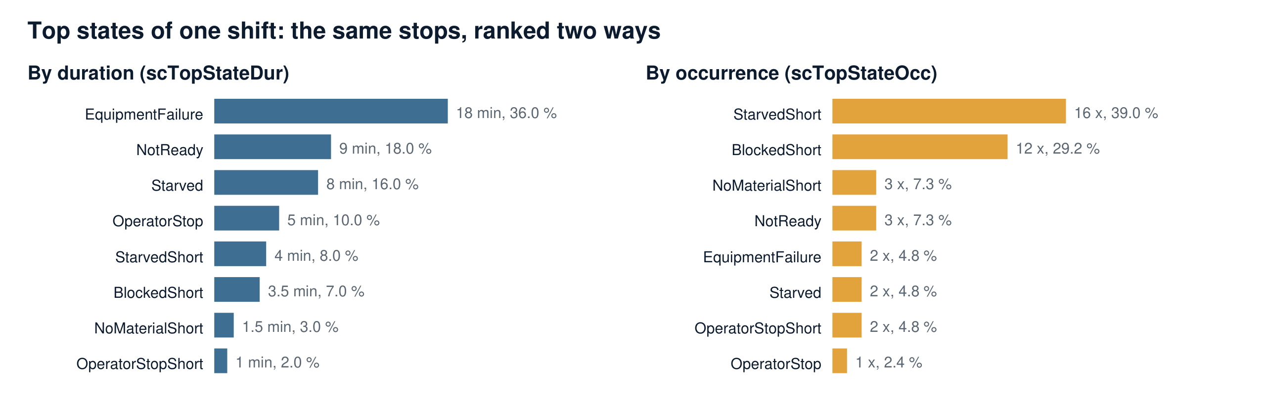
The top state analysis sorts the ten kinds of stop of the running schedule in two rankings:
by duration (scTopStateDur): position 0 is the stop that cost the most time,
by occurrence (scTopStateOcc): position 0 is the stop that happened most often.
Each entry contains the state, its duration or its count, and its share of the total in percent.
How to read it
The two rankings usually look different, and this difference is the information. In the example, failures cost the most time (36 % of the downtime in two events), while short starvation happens most often (16 of 41 stops) but costs only 8 % of the time.
The duration ranking tells you where to gain the most time. The occurrence ranking tells you what disturbs the process and the operator most often.
The percentages refer to the unplanned downtime of this schedule, not to the shift length. Breaks and NoDemand are not part of the ranking.
States without any stop are not listed; the remaining positions stay empty.
The ranking is as detailed as your state mapping (chapter 6.1). If you need the reason behind a state, for example which fault caused an EquipmentFailure, record it in the machine program next to the state.
Batch end forecast
For a batch with a target quantity the suite estimates when the batch will be finished. It does this in two steps.
Step 1: remaining build time
| Value | Formula |
|---|---|
| Remaining build time | (Batch target − products built) × ideal cycle time / OEE |
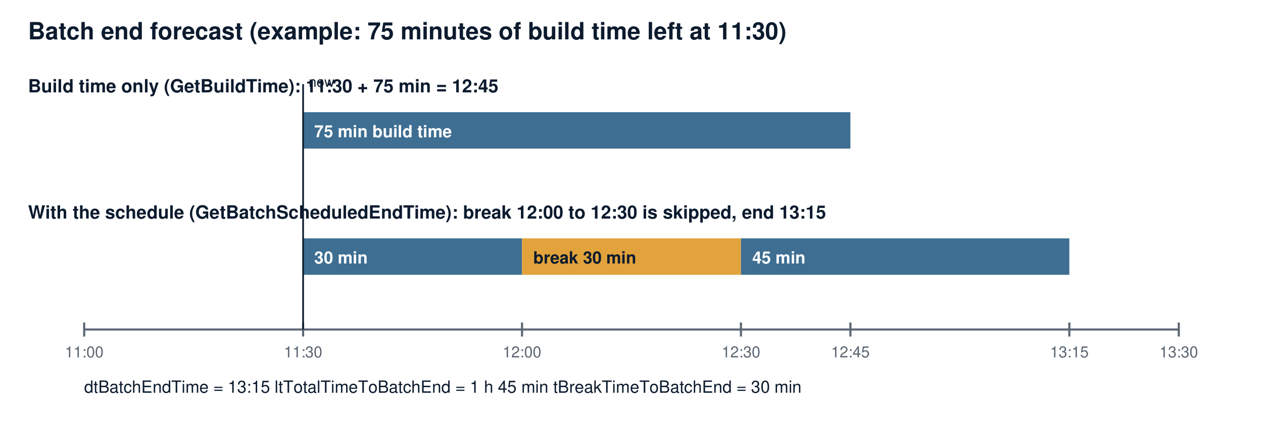
Example: target 5,000, built 1,400, planned speed 60 per minute, OEE 80 %: (5,000 − 1,400) × 1 s / 0.8 = 4,500 s = 75 minutes.
Dividing by the OEE makes the forecast realistic: a machine that reaches 80 % needs a quarter more time than the ideal. Which OEE you connect decides how the forecast behaves:
| OEE input | Behaviour of the forecast |
|---|---|
| Current OEE of the running batch | Follows what is happening now; reacts to every stop |
| Average OEE from the history | Calm; shows what is normal for this machine |
| 0 or 100 % | Ideal time without any loss; the earliest possible end |
Step 2: end time with shifts and breaks
The build time alone ignores that the machine does not produce during breaks and outside the shifts. The second step places the build time into the shift and break calendar.
| Output | Meaning | Example |
|---|---|---|
| dtBatchEndTime | Estimated date and time of the batch end | 13:15 |
| ltTotalTimeToBatchEnd | Time from now until then | 1 h 45 min |
| tBreakTimeToBatchEnd | Break time contained in it | 30 min |
| xBatchEndTimeValid | The forecast is valid | TRUE |
How to read it
The forecast is recalculated continuously. It moves later when the machine stops and earlier when it runs better than the connected OEE.
It is a forecast from the planned speed and an OEE value. It does not know about a stop that has not happened yet.
The forecast looks one week ahead. A batch that ends later is reported as an error instead of a time.
When the target is reached, xTargetReached is set.
History and results over several schedules
History. At the end of a schedule, EP_History stores its result. The last 21 schedules are available, the newest at index 0. You can compare shifts or batches with each other and pass the records on to a database.
Total result. EP_Result combines several schedules into one result, for example the three shifts of a day or the last five batches, with or without the running schedule.
Times, quantities, losses and occurrences are added up.
The KPIs are calculated again from the sums. They are not the average of the KPIs.
The top states are sorted again from the summed stops.
Why not simply the average? Two shifts:
| Planned production time | Run time | Availability | |
|---|---|---|---|
| Shift 1 | 420 min | 399 min | 95 % |
| Shift 2 (short, with a long failure) | 120 min | 60 min | 50 % |
| Average of the two percentages | 72.5 % | ||
| Calculated from the sums | 540 min | 459 min | 85 % |
The average treats the short shift like the long one. The result from the sums is the availability the machine really had in these nine hours.
When a value looks unexpected
| Observation | Explanation | What to do |
|---|---|---|
| Performance stays at 100 % at the start of a shift | Start-up phase (chapter 5.4) | Wait, or shorten the start-up time and count |
| Performance is above 100 % | Planned speed is lower than the real speed | Correct products per minute |
| Performance is low although the machine "ran all the time" | The planned speed is the technical maximum, or short stops are not reported as stops | Check products per minute and the state mapping |
| Performance loss goes down and availability loss goes up | A stop has passed the short stop time (chapter 6.2) | Nothing; intended |
| KPIs change only every few seconds | Update filter (chapter 5.4) | Adjust tKPIUpdateFilter |
| OEE is 0 | One factor is 0, usually before the first part | Wait for the first parts |
| Quantity is above 0 right at the start of a shift | Parts were produced before the shift started (chapter 3) | Nothing; they do not count for the performance |
| Top states show only one or two states | The machine program reports only these states | Refine the state mapping |
| Availability of a day differs from the average of its shifts | Results over several schedules are calculated from the sums (chapter 10) | Nothing; the result from the sums is correct |
| Batch end time jumps | The current OEE is connected (chapter 9.1) | Use an average OEE for a calmer forecast |
| Values are cleared at the shift change | A new schedule starts at zero (chapter 3) | Use the history or EP_Result |
| Durations jump by one hour | The clock was changed, for example daylight saving time; durations follow the local time | Only the schedule during the change is affected |
| xError is TRUE and iErrorID is set | A parameter is missing or out of range | See the error table in the library manual |
Terms
| Term | Meaning |
|---|---|
| Schedule | Period that is evaluated: a shift, a batch or a product run |
| All time | Time since the schedule started |
| Schedule loss | Time without planned production: breaks, no demand |
| Planned production time | All time minus schedule loss |
| Run time | Planned production time minus availability loss |
| Net run time | Run time minus short stops and speed loss; equal to ideal cycle time × total count |
| Ideal cycle time | Time for one product at planned speed |
| Short stop | Stop shorter than the configured short stop time; performance loss |
| Long stop | Every other stop; availability loss |
| Speed loss | Output lost because the machine ran slower than planned |
| OEE | Overall Equipment Effectiveness: availability × performance × quality |
| TEEP | Total Effective Equipment Performance: OEE × planned production time / all time |
| Top state | Kind of stop in the ranking by duration or by occurrence |
References
OEE definitions and calculation: https://www.oee.com/calculating-oee/
OEE factors and time model: https://www.oee.com/oee-factors/
Six Big Losses: https://www.oee.com/oee-six-big-losses/
World-class OEE: https://www.oee.com/world-class-oee/
Function blocks, structures and error codes: DDAS Date Time, Scheduler and Equipment Performance Library Manuals, https://ddas.cloudet.digital
Your Feedback Matters
These instructions have been prepared to the best of our knowledge and belief to provide you with the highest possible level of support when working with our product.
If you identify any issues or have suggestions for improvement, we would greatly appreciate your feedback. Please send your comments in a short e-mail to:
Thank you for your support.
Your DDAS Application Software Team